%pylab inline
from pyiga import bspline, geometry, vis

Populating the interactive namespace from numpy and matplotlib

Geometry manipulation in pyiga

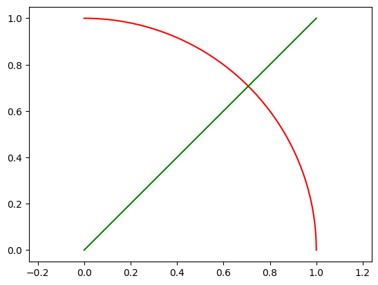
We can define line segments or circular arcs using the builtin functions from the geometry module (see its documentation for details on all the functions used here). All kinds of geometries can be conveniently plotted using the vis.plot_geo() function.

f = geometry.circular_arc(pi/2)
g = geometry.line_segment([0,0], [1,1])

vis.plot_geo(f, color='red')
vis.plot_geo(g, color='green')
axis('equal');

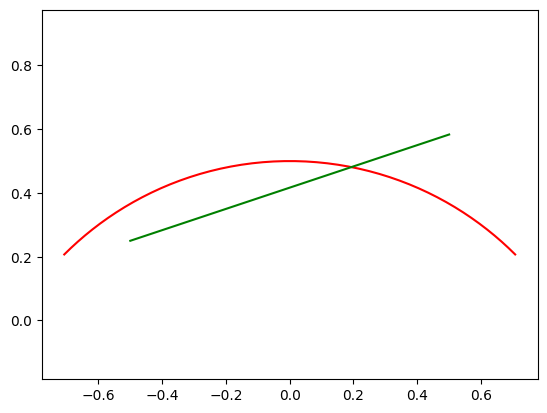
Geometries can be translated, rotated or scaled:

vis.plot_geo(f.rotate_2d(pi/4).translate([0,-0.5]), color='red')
vis.plot_geo(g.scale([1,1/3]).translate([-.5,.25]), color='green')
axis('equal');

We can combine the univariate geometry functions \(f(y)\) and \(g(x)\) to create biviariate ones using, for instance, the outer sum

\[(f \oplus g)(x,y) = f(y) + g(x)\]

or the outer product

\[(f \otimes g)(x,y) = f(y) * g(x).\]

Here, both the addition and the product have to be understood in a componentwise fashion if \(f\) and/or \(g\) are vector-valued (as they are in our example).

vis.plot_geo(geometry.outer_sum(f, g))
axis('equal');

vis.plot_geo(geometry.outer_product(f, g))
axis('equal');

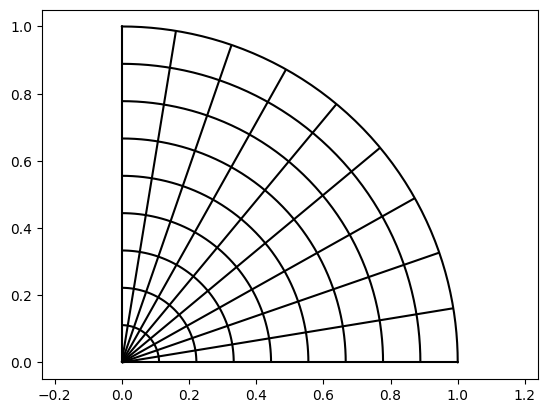
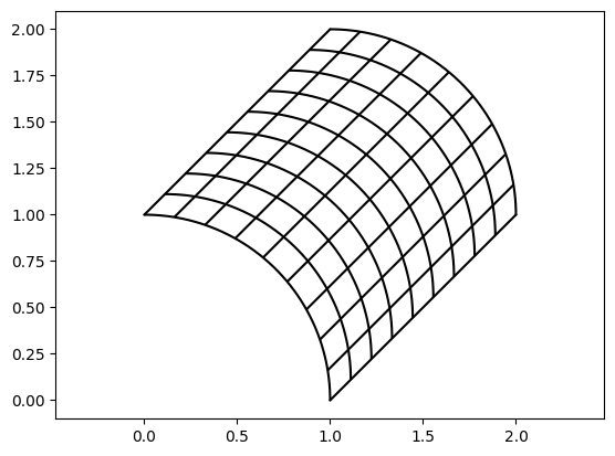
The last outer product has a singularity at the origin because multiplying with \(g(0)=(0,0)\) forces all points into \((0,0)\). We can translate it first to avoid this, creating a quarter annulus domain in the process:

vis.plot_geo(geometry.outer_product(f, g.translate([1,1])))
axis('equal');

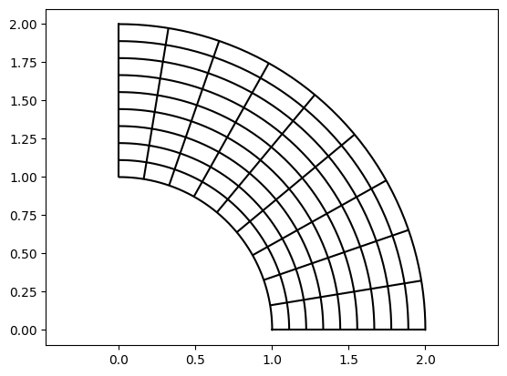
In this example, the second operand was a line segment from \((1,1)\) to \((2,2)\). Since numpy-style broadcasting works for all these operations, we can also simply define the second operand as a linear scalar function ranging from 1 to 2 to obtain the same effect:

vis.plot_geo(geometry.outer_product(f, geometry.line_segment(1, 2)))
axis('equal');

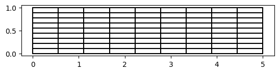
We can also generate tensor product geometries; here each input function \(f\) and \(g\) has to be scalar such that the resulting output function \(F\) is 2D-vector-valued, namely,

\[F(x,y) = (g(x), f(y)).\]

However, you can also use this with higher-dimensional inputs, for instance to build a 3D cylinder on top of a 2D domain.

G = geometry.tensor_product(geometry.line_segment(0,1),
                            geometry.line_segment(0,5, intervals=3))
vis.plot_geo(G)
axis('scaled');

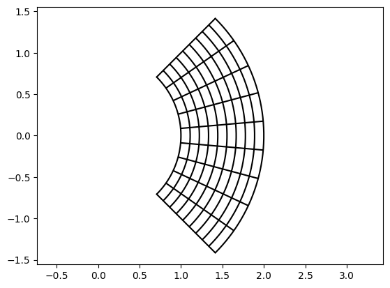
We can also define geometries through user-defined functions, where we have to specify the domain:

def f(x, y):
    r = 1 + x
    phi = (y - 0.5) * np.pi/2
    return (r * np.cos(phi), r * np.sin(phi))

f_func = geometry.UserFunction(f, [[0,1],[0,1]])
vis.plot_geo(f_func)
axis('equal');

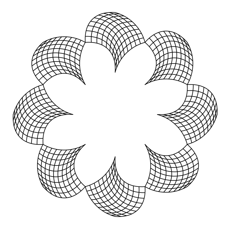
Finally, a bit of fun with translated and rotated outer products of circular arcs:

figsize(10,10)
G1 = geometry.circular_arc(pi/3).translate((-1,0)).rotate_2d(-pi/6)
G2 = G1.scale(-1).rotate_2d(pi/2)
G1 = G1.translate((1,1))
G2 = G2.translate((1,1))

G = geometry.outer_product(G1, G2).translate((-1,-2)).rotate_2d(3*pi/4).translate((0,1))

for i in range(8):
    vis.plot_geo(G.rotate_2d(i*pi/4))
axis('equal');
axis('off');